Generation, Propagation, and Spectra of Atmospheric Gravity Waves

1. What are Atmospheric Gravity Waves?

Atmospheric gravity waves, also known simply as gravity waves, are one of the main components of atmospheric waves, whose restoring force is buoyancy in the atmosphere. Although the name is similar to gravitational waves, appearing in the context of the general theory of relativity, they are completely different types of waves.

Although buoyancy may sound difficult to understand, there is no need to worry. Suppose a small parcel of the air is lifted upward to a certain height (left side of Fig. 1-1). The air pressure decreases, and thus the parcel expands slightly. In most cases concerning the atmosphere, the density of the parcel is higher than that of the surrounding air. Thus, the parcel returns toward its original position because it receives a downward buoyancy. Since it gained potential energy as it was lifted, it will overshoot the original, balanced position and move further downward. Then, the buoyancy applied to the parcel becomes upward, and it rises to the original position again. However, it does not stop there, but rather overshoots this position and moves further upward. If there is no friction, this oscillation repeats. This is called buoyancy oscillation.

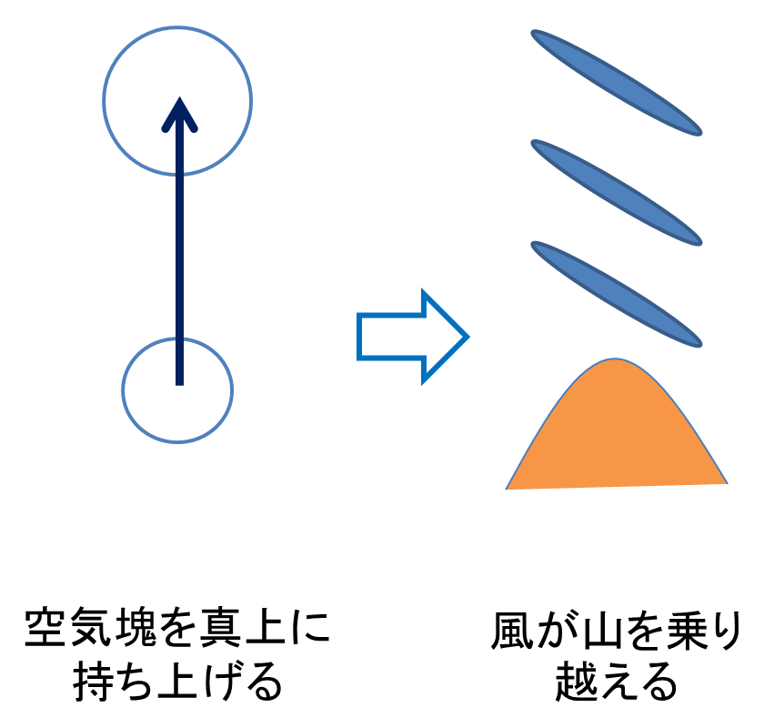
**Figure 1-1** Schematic diagram of buoyancy oscillations and atmospheric gravity waves. The arrow in the right panel represents the direction of the background wind, and the blue diagonal ellipses represent the phase of a gravity wave.

In buoyancy oscillation, the parcel of the air oscillates vertically. On the other hand, in atmospheric gravity waves, the air mass oscillates diagonally (Fig. 1, right). The buoyancy is caused by gravity, which is why it is called a gravity wave. For buoyancy to work, the parcel must be lifted in the direction of gravity (i.e., vertically). This happens, for example, when the wind rises over a mountain. Gravity waves are also generated by phenomena that involve strong vertical motion, such as cumulus clouds. Additionally, gravity waves are excited when water vapor repeatedly forms clouds while emitting latent (condensation) heat. Other interesting mechanisms in atmospheric dynamics, such as gravity waves generated by large-scale jet streams, will be discussed later.

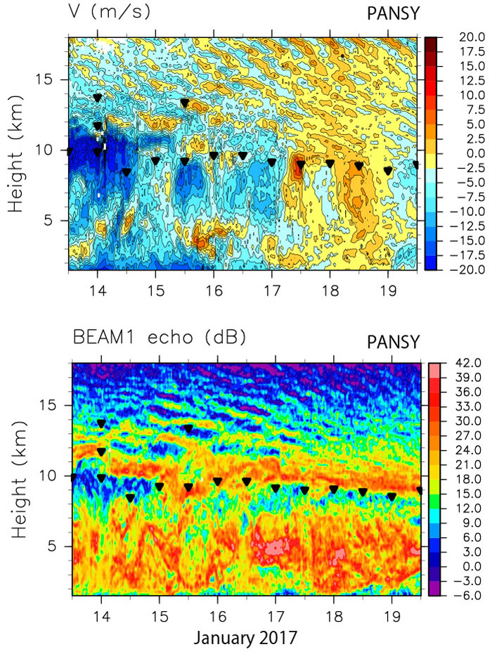
Figure 1-2 shows observational data (14–20 January 2017) acquired by the PANSY radar, the first large-scale atmospheric radar in the Antarctic, which is installed at Syowa Station. The upper and upper panels show the time–height cross sections of the meridional wind and intensity of scattered radio waves, called echo intensity, received by the radar, respectively. The echo intensity reflects the intensity of turbulence and stratification of the atmosphere. Wave-like structures propagating downward over time can be seen in both panels. These are gravity waves.

**Figure 1-2** Meridional wind (top) and echo intensities of vertical beams (bottom) observed by the PANSY radar during 14–20 January, 2017. ▼ is the height of the tropopause.

2. History of Atmospheric Gravity Wave Research

Gravity waves do not directly affect daily weather very much because of their small spatial scales and weak amplitudes in the troposphere. Hence, apart from theoretical studies concerning purely the interests of atmospheric dynamics, they were treated as "weather noise." However, since the beginning of the 1980s, the development of advanced observation methods, such as large-scale atmospheric radar, and rapid progress in computer technology clarified the nature of these waves, and their importance was recognized theoretically. Although most weather and climate forecast models lacked sufficient resolutions to represent gravity waves, effects of gravity waves are included in these models as parameters based on scientific knowledge at that time (called parameterization methods). In the 1990s, the focus shifted to the tropics, and since the beginning of the 2000s, the focus has expanded to the polar regions, and to global characteristics and behaviors of gravity waves. These days, observations and collaborative research have been conducted globally.

Moreover, gravity waves cause upward and downward flows strong enough to affect aircraft. It has recently been shown that they cause extreme weather phenomena such as torrential rains. It is currently extremely difficult to predict gravity waves themselves, but further research must be conducted from the perspective of disaster mitigation.

1980s The Era of the Mid-Latitudes: More Accurate Weather Forecasts
It was shown that gravity waves maintain the weak wind layers at the mid-latitude mesopause and in the lower stratosphere. The incorporation of this gravity wave effect into forecast models greatly improved the accuracy of weather forecasts.
1990s The Era of the Tropics: Atmospheric Gravity Waves Driving Large-Scale Atmospheric Oscillations
Awareness of the importance of atmospheric gravity waves was further enhanced by the findings that they and similar types of waves are the driving forces behind the quasi-biennial, large-scale, atmospheric oscillations in the equatorial lower stratosphere.
2000 - Present The Era of the Polar Region: A Comprehensive Understanding of the Global Atmosphere
Atmospheric general circulation models that can resolve gravity waves can now be run on supercomputers. In addition, high-resolution satellite observations that measure temperature fluctuations associated with gravity waves have advanced. These developments of technologies allow us to capture global gravity wave activity. Moreover, it is revealed that gravity waves in the polar regions significantly contribute to improving the accuracy of weather forecast models (i.e., these waves have properties that are totally different from our predictions at that time), and thus, thorough observation and research of gravity waves in the polar regions are required. Furthermore, the atmosphere at the north and south poles may be modulated almost simultaneously (i.e., teleconnection) due to global changes in the propagation and wave forcing of gravity waves in the mesosphere.

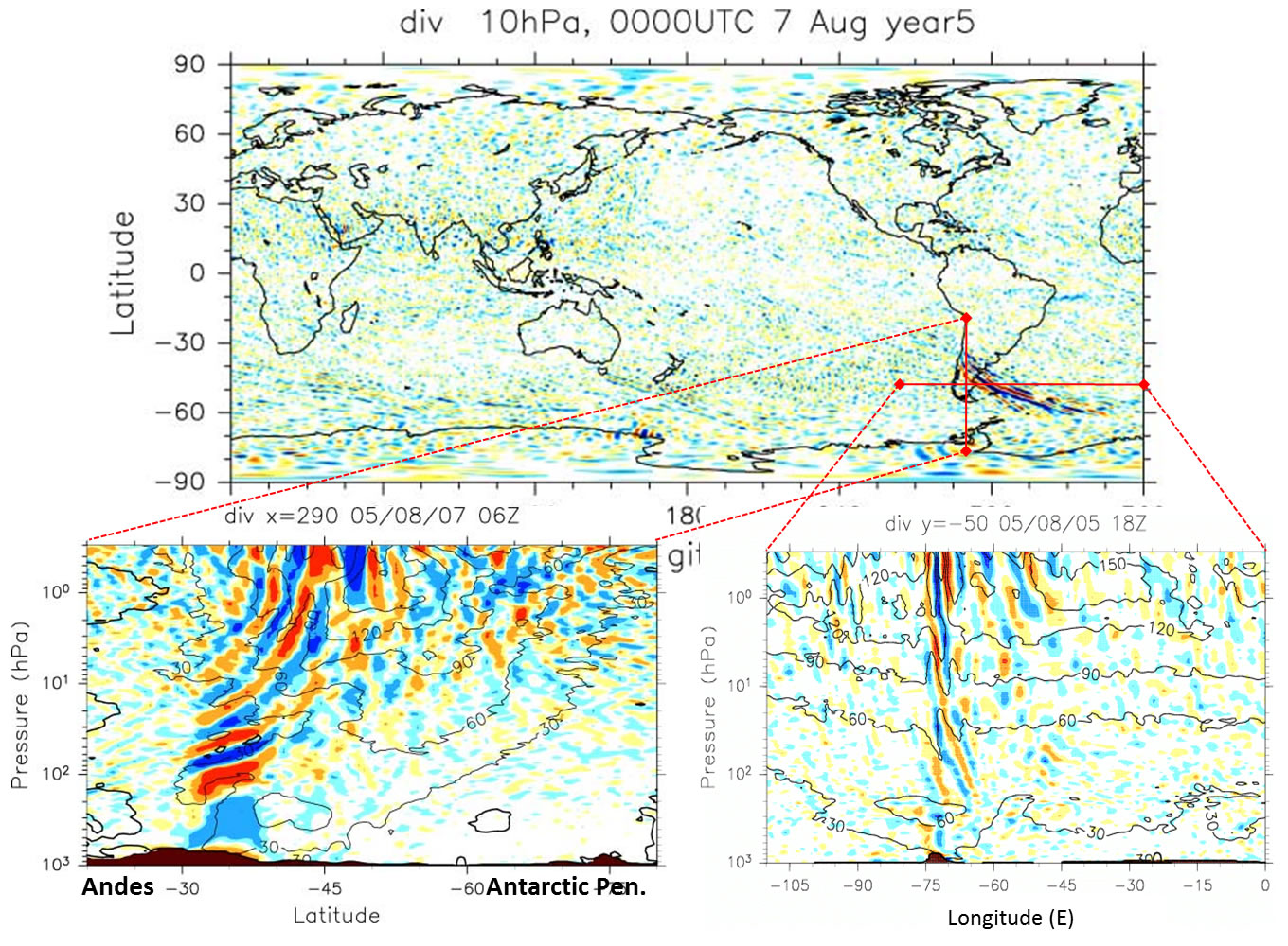
Figure 2-1 shows gravity waves simulated by our world-leading high-resolution atmospheric general circulation model with realistic (but not real) boundary conditions such as sea surface temperature, wherein a quantity called horizontal divergence is plotted. Since horizontal divergence associated with Rossby waves is almost zero, we can see gravity waves by plotting the horizontal divergence with no need to extract small-scale components. Gravity waves look like fine dots. The figure shows that strong gravity waves are emitted from the Andes Mountains in South America. Gravity waves with large amplitudes are also excited around the Asian monsoon, where convection is active; around the Southern Ocean, where there is strong cyclone activity; and around the Antarctic Continent.

We have been studying atmospheric gravity waves using various methods including observation, model simulation, mass data analysis, and theoretical approach. Currently, we are conducting research using a pioneering atmospheric general circulation model that resolves gravity waves. Another ongoing research topic is full-scale polar gravity wave observations obtained by the first large-scale atmospheric radar (PANSY radar) at Syowa Station in the Antarctic. In addition, in collaboration with researchers from other countries, we are conducting research to elucidate the mechanisms of global climate teleconnection by combining simultaneous observations of gravity waves and their global modification with hindcast simulations performed by atmospheric general circulation models.

**Figure 2-1** Global map of gravity waves at 10 hPa (approximately 30 km in altitude) reproduced by the gravity-wave-permitting atmospheric general circulation model, and the latitudinal and longitudinal-height cross sections along the red lines. Red (blue) represents divergence (convergence) of horizontal wind. Snapshot in August.

3. Lateral Propagation of Atmospheric Gravity Waves

Atmospheric gravity waves oscillate (diagonally) upward and downward; thus, the direction of their energy propagation can be considered nearly vertical compared to Rossby waves. In addition, the velocity of upward energy propagation (vertical group velocity) is larger than that of Rossby waves. For example, it takes less than one hour for gravity waves originating at a mountain (mountain waves) to reach the tropopause, which is about 10 km from the ground. Thus, the parameterization used in many weather and climate forecast models are based on the assumption that gravity waves propagate only vertically upward and instantaneously.

However, gravity wave oscillation can be nearly horizontal, depending on the strength of the background wind and stratification of the atmosphere. In such a case, it is usual that gravity waves take many days to reach the top of the neutral atmosphere at 100 km. In addition, gravity waves propagate not only vertically, but also horizontally. For example, gravity waves originating at the Southern Andes, as shown in Fig. 2-1, appear to be advected eastward, and in fact it is theoretically explained that energy of gravity waves is transported eastward.

Although the horizontal propagation of gravity waves did not use to attract much attention, it cannot be neglected, considering the effects of gravity waves on the mean flow.

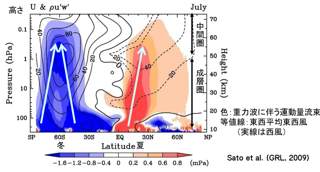
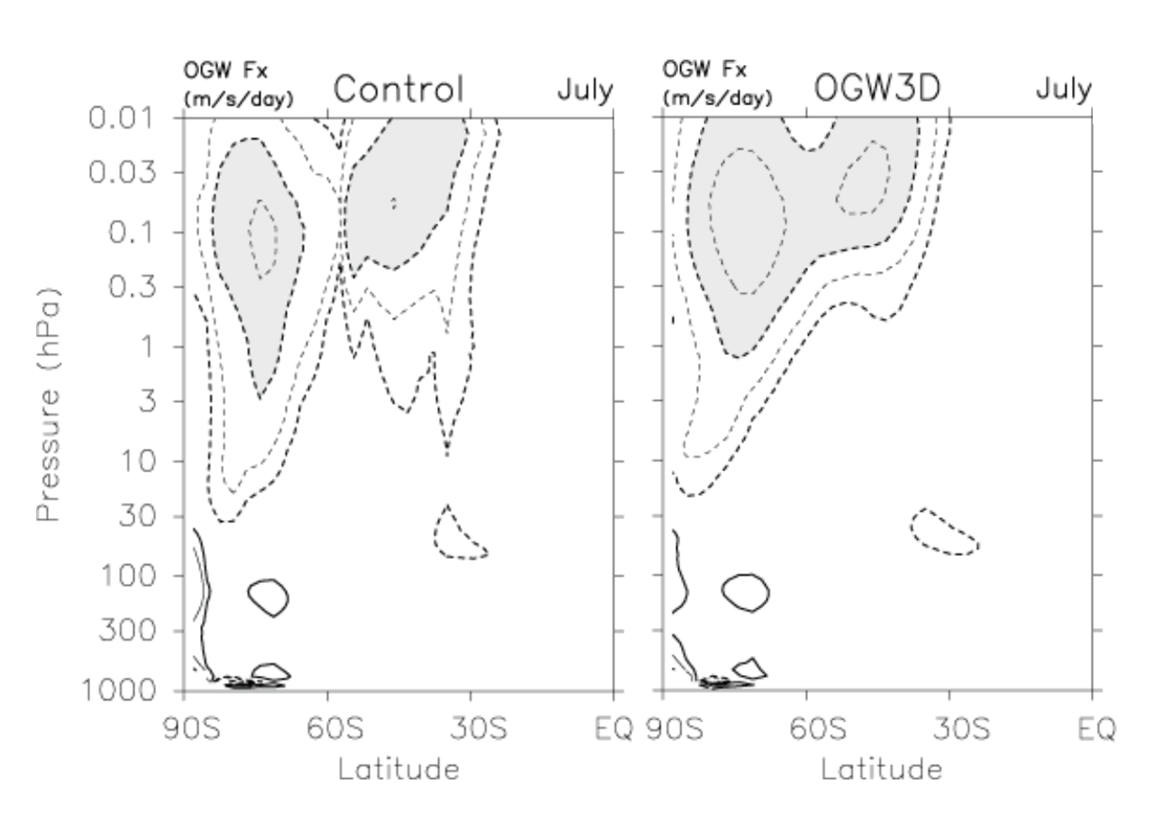
**Figure 3-1** Momentum fluxes (colors) and mean zonal winds (contours) associated with gravity waves simulated by the gravity-wave-permitting atmospheric general circulation model. Solid contours represent eastward winds; dashed contours represent westward winds (Sato et al., 2009).

Figure 3-1 shows the latitude-height section of the momentum carried by gravity waves (called momentum flux) reproduced by the gravity-wave-permitting atmospheric general circulation model (same data as Fig.2-1). Red represents the vertical flux of the eastward momentum and blue represents that of westward momentum. Positive (solid) contours indicate eastward winds, and negative (dashed) contours indicate westward winds. The momentum flux of gravity waves is conserved unless the waves are broken or attenuated by atmospheric friction. Therefore, this distribution implies that gravity waves propagate not only vertically but also laterally (latitudinally) as shown by the light blue arrows.

There are two possible mechanisms for horizontal propagation. The first is the refraction of gravity waves. As can be seen from the contours in Fig.3-1, there is a strong eastward jet (called the polar night jet) in the winter hemisphere, and a strong westward jet in the summer hemisphere. In other words, there is latitudinal shear in the background wind where gravity waves propagate. This shear refracts gravity waves and causes them to propagate horizontally.

The second is advection caused by background wind. Advection is the effect of being swept downstream by the background wind. Solution of the two-dimensional (horizontal and vertical) theory shows that for mountain waves, only the vertical group velocity is large, whereas the horizontal group velocity is almost zero. A gravity wave packet has an intrinsic group velocity in the direction of the wavenumber vector, which is perpendicular to the ridge of a mountain chain in the case of mountain waves. The intrinsic horizontal group velocity of a mountain wave packet is the same magnitude as that of the background flow in the opposite direction. Hence, the net horizontal group velocity (i.e., the group velocity relative to the ground) is zero when the background flow is considered. This is the theoretical basis for the assumption of only vertical propagation in gravity wave parameterizations.

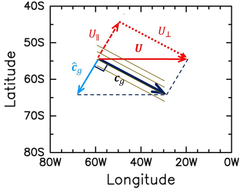
However, the real atmosphere is three-dimensional. In such case, the net horizontal group velocity is zero only in the direction parallel to the wavenumber vector ( in Fig. 3.2). The wave packet has no group velocity to cancel the advection by the background wind perpendicular to the wavenumber vector . Thus, the energy of the gravity wave packet is swept downstream in this direction. In other words, even gravity waves originating at a mountain are advected.

**Figure 3-2** Advection of orographic gravity waves by the background wind.

Moreover, we have shown that not only does the refraction of gravity waves result in horizontal propagation of them, but the refraction itself imposes a non-negligible forcing on the mean wind.

**Figure 3-3** Gravity wave forcing attributable to refraction (the left side is without refraction; the right side is with refraction) from Amemiya and Sato (2015).

4. Sources of Gravity Waves

There are various sources of atmospheric gravity waves. At mid- and high latitudes, topography (such as mountains) and jet streams and fronts in the troposphere are the main sources, whereas at low latitudes, the main source is active convection.

a. Jet Streams and Mountains

At Syowa Station in the Antarctic, multiple tropopauses are often observed. During winter, quadruple and quintuple tropopauses are not unusual. However, the reason for this has been unclear. Using observational data from the PANSY radar at Syowa Station, we found that strong inertial gravity waves exist in the lower stratosphere, and large-amplitude temperature fluctuations associated with these waves are detected as tropopauses.

The animation below shows the generation and propagation of gravity waves in the polar regions of the Southern Hemisphere as simulated by a numerical model during the period when multiple tropopauses were observed. The validity of the model was confirmed by comparison with the PANSY radar data. The animation shows that gravity waves are generated and propagated above the sea and near the Antarctic coastline. Their group velocities and phase characteristics, as well as the structure of the background wind, indicate that gravity waves near the coastline likely originated from the steep slopes along the Antarctic coast, while those above the sea likely originated from the meandering polar front jet (Shibuya et al., 2015).

Figure 4-1 Animation showing horizontal divergence in the horizontal map at a height of 17.5km (left) and latitude–height section at 65°S (right). The simulation period was four days (7–10 April 2014).

b. Spontaneous Adjustment Process of Balanced Flow (Quasi Resonance Theory)

As previously mentioned, gravity waves are typical waves of unbalanced flows. In contrast, an extratropical cyclone is an example of a balanced flow. However, in the mid-90s, an astonishing theory in atmospheric dynamics proposed that gravity waves are emitted from extratropical cyclones. The gravity wave over the Southern Ocean seen in Fig. 2-1 may have been generated through such a mechanism.

This type of gravity wave generation is called spontaneous radiation, and many theoretical studies have examined its mechanisms. The mainstream theory states that the balance of a balanced flow (the balance between the Coriolis force and the pressure-gradient force) can be broken due to the nonlinearity of the fluid equations. Subsequently, gravity waves are generated when the flow becomes balanced again. We have proposed a new theory in response to this idea.

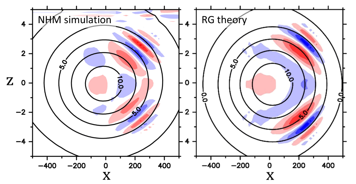
Gravity waves have intrinsic frequencies (frequencies relative to the background wind) that are significantly higher than the time scales of balanced flows. Thus, unbalanced and balanced flows hardly interact due to the large difference between their frequencies. However, if the balanced flow is strong enough to cause a large Doppler shift in the frequency of the gravity waves, their apparent periods (periods relative to the ground) may extend to match that of the balanced flow. Our new theory states that, in these cases, resonance occurs between the balanced flow and the gravity waves, and gravity waves are generated. Figure 4-2 compares the theoretical calculations for gravity waves generated by the renormalization group method (right panel of Fig.4-2) with a simulation of gravity wave generation by a jet (left panel of Fig.4-2). The similarity of gravity wave structure in these two panels confirms our theory that gravity waves are generated by resonance with a balanced flow.

In the 1980s, large-scale atmospheric radar observations revealed that the periods of gravity waves emitted from jets are very long. This fact can be explained by this theory. Furthermore, it can also explain the characteristics of transient spontaneous radiation: When energy is transferred to gravity waves by resonance, the balanced flow is decelerated. As a result, resonance between gravity waves and the balanced flow ceases, and gravity wave radiation stops.

We propose that this is the essence of spontaneous radiation. Interestingly, the forcing induced by gravity wave radiation derived from the resonance theory is similar to that described by the deviation from the balanced flow, which was considered in previous studies (e.g., Plougonven and Zhang, 2007; Snyder et al. 2009; Wang and Zhang 2010). This result confirms the physical validity of the previous studies of spontaneous radiation.

**Figure 4-2** East–west height cross section of the strength of the eastward jet (contours) and the generated gravity waves (horizontal wind divergence (convergence) is denoted by red (blue) shadings) (Yasuda et al., 2015).

c. Inertial Oscillations in the Boundary Layer

We have also found a mechanism for the generation of gravity waves that has not been noted previously. By simulating the atmospheric boundary layer with daily variations in solar radiation, we found that the amplitudes of the inertial oscillations in the nighttime boundary layer increase at latitudes of 30 degrees and 90 degrees, where the periods of inertial oscillations coincide with the diurnal and semidiurnal period, respectively. This can be understood as a quasi-resonance phenomenon between the inertial oscillations and the daily variations in solar radiation. Gravity waves having periods close to the inertial period are excited at the upper edge of the atmospheric boundary layer.

**Figure 4-3** Time–height cross section of zonal wind in the boundary layer at 30 degrees latitude, which shows a fluctuation having a daily period. The period of such fluctuations varies depending on the latitude, which is 16 hours at 60 degrees and 12 hours at 90 degrees. At 30 degrees latitude, since the inertial period is one day, resonance occurs. The upper edge of the boundary layer, where the amplitude of the zonal wind fluctuation increases, is a height of about 1,200 m. Above this layer, inertial gravity waves are observed, whose phase descends with time (Shibuya et al. 2014).

5. Gravity Wave Spectrum

As previously mentioned, higher resolutions of atmospheric general circulation models now enable us to simulate gravity waves. However, model-simulated atmospheres are only a virtual world, which may differ from the real atmosphere. Thus, they must be validated with high-resolution observational data. Because of difficulty in gravity wave observation, observational data available for verifying gravity waves in a model is limited. We compared our model simulations with MU radar observations, which are one of the representatives of large-scale atmospheric radars at mid-latitudes.

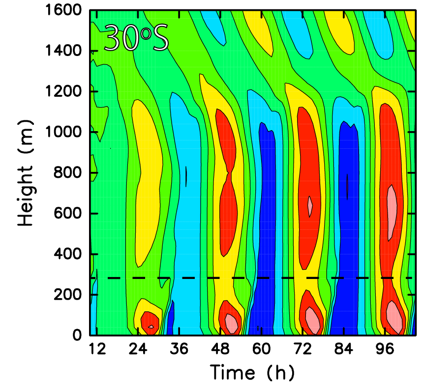
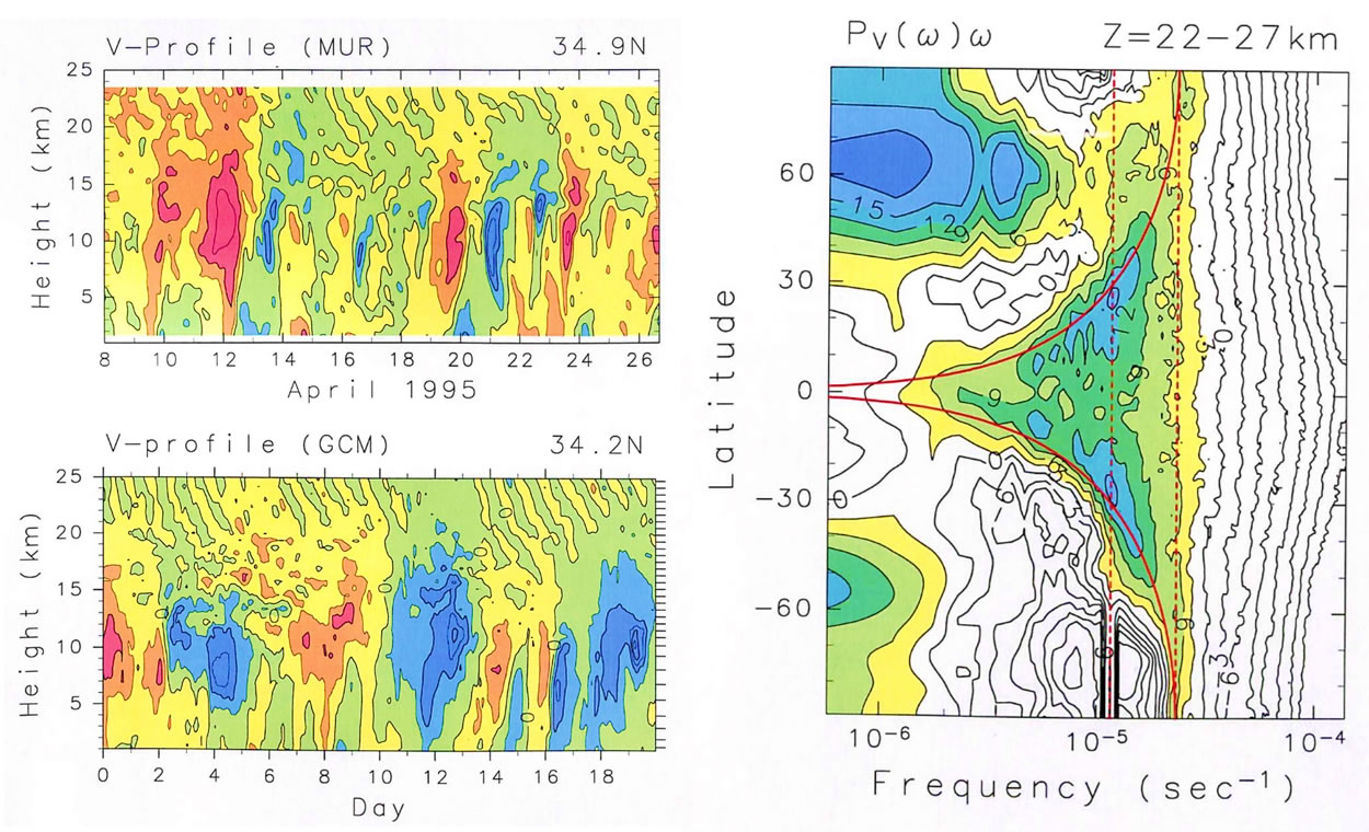
The left side of Fig. 5-1 shows a time–height cross section for the meridional wind, with the upper panel showing MU radar observations and the lower panel showing a simulation result using the atmospheric general circulation model. These figures show a wave-like structure, the phase of which descends over time, above a height of 20 km. The period, vertical wavelength, and amplitude all correspond well. This fact supports that the model reproduced gravity waves very well.

Next, utilizing the capabilities of the model, we examined the variations in the frequency power spectrum with latitude (right side of Fig.5-1). The red dotted line on the left (right) indicates the one-day (half-day) period. The solid red curves indicate the inertial period at each latitude. A peak of the spectrum is observed at approximately the inertial period at almost all latitudes, except near the equator, where the inertial period is infinite. Around a latitude of 35 degrees, where the MU radar is located, there is a peak at approximately 20 hours. This is not a peak observed at a daily period due to the rotation of the Earth, but rather observed at the inertial period, which is approximately 21 hours at 35 degrees.

**Figure 5-1** Meridional wind from three-week continuous observations by the MU radar (upper left) and a 20-day simulation using a gravity-wave-permitting atmospheric general circulation model (lower left). The right panel shows the frequency spectrum of the meridional wind calculated using the general circulation model. The vertical axis shows the latitude. The solid red curves represent the inertial frequency. The dotted red line indicates the 24-hour period on the left and the 12-hour period on the right (Sato et al., 1999).

The possible intrinsic periods (periods observed from the background flow) of gravity waves range from the period of buoyancy oscillation to the inertial period. The buoyancy oscillation period is approximately 10 minutes in the troposphere and approximately 5 minutes in the middle atmosphere. The inertial period is a function of latitude only; for example, it is 24 hours at 30 degrees latitude and 12 hours at the poles (solid red curves in the right panel of Fig.5-1). Thus, the frequency range of gravity wave is very wide. There is a dearth of long-term data available for investigation of the spectrum of this entire range, except for near the ground. In addition, the vertical wavelengths of gravity waves range from a few hundred meters to infinity. Thus, observations with a high vertical resolution are necessary to obtain gravity wave spectra.

The PANSY radar, which is the Antarctic large-scale atmospheric radar, has been continuously observing since May 2012. Large-scale atmospheric radars can observe the troposphere, stratosphere, and mesosphere with high vertical and time resolutions. However, they can only receive echoes during the day, when solar radiation is present. In the Antarctic region, solar radiation exists continuously during summer due to the midnight sun. Moreover, polar mesospheric clouds are formed during this period, causing strong echoes known as polar mesospheric summer echoes (PMSE), that are continuously received. Thus, we can observe the mesosphere almost continuously over many days during the summer in the polar region.

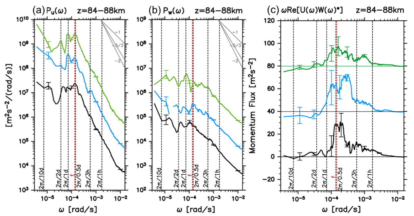
**Figure 5-2** Frequency power spectra of the (a) zonal wind and (b) vertical wind in the mesosphere at an altitude of 84–88 km. The horizontal axis shows the period range from 8 minutes to 20 days. (c) Frequency spectra of vertical fluxes of zonal momentum. Green (top), blue (middle), and black (bottom) curves show the data from the summer of 2015–16, 2014–15, and 2013–14, respectively (Sato et al., 2017).

Figures 5-2(a) and (b) show the frequency (ω) spectra of the horizontal and vertical winds in the mesosphere, respectively. The horizontal (vertical) wind spectra have a shape that is proportional to ω^-2 (ω^-1) at periods shorter than the inertial period, that is, approximately 13 hours. Momentum flux associated with gravity waves can be accurately estimated using large-scale atmospheric radar observations. Figure 5-2(c) shows the spectra of these fluxes. Although it used to be generally assumed that gravity waves having short periods have large momentum fluxes, it was found that the gravity waves having long periods (1 hour to 1 day) have large momentum fluxes.

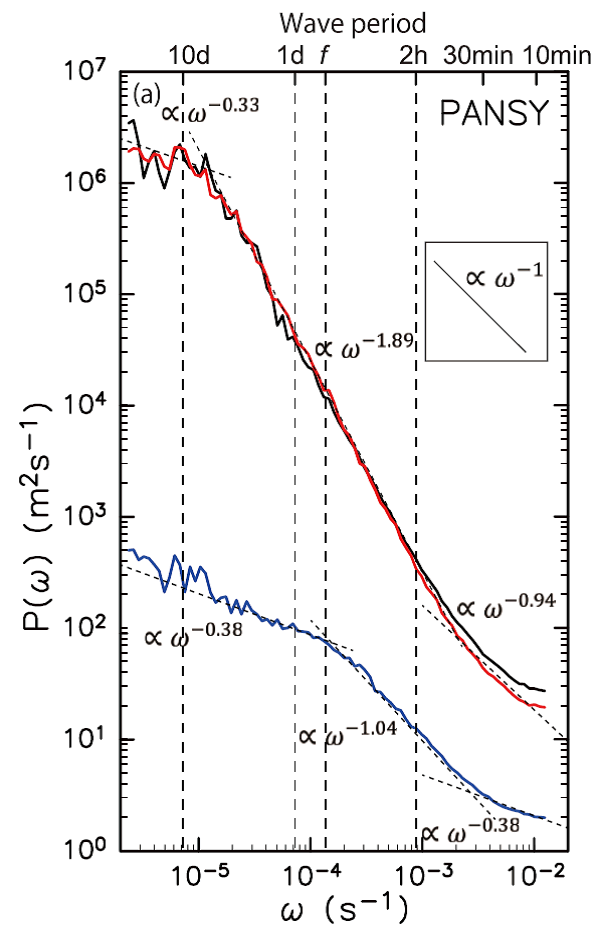
Figure 5-3 shows the frequency spectrum in the lower troposphere as observed by the PANSY radar. The black curve represents the zonal wind spectrum, red represents the meridional wind spectrum, and blue represents the vertical wind spectrum. The vertical wind spectrum has a similar shape to that of the mesosphere. Although the horizontal wind spectrum has a shape nearly proportional to ω^-2, the longer end of the period range proportional to ω^-2 is approximately 7 days, which is longer than that of the mesosphere.

It is interesting that, unlike the mesosphere, the energy in the long period range, from the inertial period to seven days, is very large in the lower troposphere when compared with that in the shorter period range. Because gravity waves have shorter periods than the inertial period, the waves that compose this long period range are not gravity waves. It is suggested that the reason for the difference between spectra in the lower troposphere and mesosphere is that small-scale (i.e., not planetary-scale) Rossby waves cannot propagate through the stratosphere, whose theoretical background lies in the Charney and Drazin theorem.